The History of Numerical Weather Prediction
Numerical weather prediction involves the use of mathematical models of the atmosphere to predict the weather. Manipulating the huge datasets and performing the complex calculations necessary to do this on a resolution fine enough to make the results useful is the responsibility of NOAA’s National Centers for Environmental Prediction (NCEP). NCEP delivers national and global weather, water, climate, and space weather guidance, forecasts, warnings, and analyses needed to help protect life and property, enhance the nation's economy, and support the nation's growing need for environmental information.
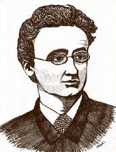
Vilhelm Bjerknes was a professor of applied mechanics and mathematical physics at the University of Stockholm, where his research revealed the fundamental interaction between fluid dynamics and thermodynamics.
The roots of numerical weather prediction can be traced back to the work of Vilhelm Bjerknes, a Norwegian physicist who has been called the father of modern meteorology. In 1904, he published a paper suggesting that it would be possible to forecast the weather by solving a system of nonlinear partial differential equations.
A British mathematician named Lewis Fry Richardson spent three years developing Bjerknes’s techniques and procedures to solve these equations. Armed with no more than a slide rule and a table of logarithms, and working among the World War I battlefields of France where he was a member of an ambulance unit, Richardson computed a prediction for the change in pressure at a single point over a six-hour period. The calculation took him six weeks, and the prediction turned out to be completely unrealistic, but his efforts were a glimpse into the future of weather forecasting.
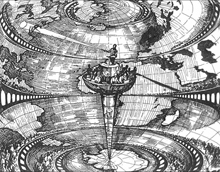
This illustration depicts Richardson’s “forecast factory.” Click image for larger view and image credit.
Richardson foresaw a “forecast factory,” where he calculated that 64,000 human “computers,” each responsible for a small part of the globe, would be needed to keep “pace with the weather” in order to predict weather conditions. They would be housed in a circular hall like a theater, with galleries going around the room and a map painted on the walls and ceiling. A conductor located in the center of the hall would coordinate the calculations using colored lights...
While Richardson’s vision never became a reality, the use of mathematics to predict the weather did develop over the years. This article looks at the evolution of a science that NOAA uses everyday to deliver the weather forecasts upon which we have come to rely on.
The Early Evolution of Numerical Weather Predictions
Several decades passed after Richardson’s initial efforts in numerical weather prediction. During this time, meteorological observation, research, and technology struggled to reach the level necessary to make the computations envisioned by Richardson.
Small, yet significant, milestones were reached during the early part of the 20th century. The first meteorological radiosonde, a balloon carrying instruments to measure atmospheric temperature, pressure, humidity, and winds, was launched in the United States in 1937. In World War II, American pilots over the South Pacific felt the effects of the jet stream, a current of fast-moving air found in the upper levels of the atmosphere whose presence had previously only been theorized. Communication technology grew to allow hundreds of meteorological observations to be collected from around the globe. Most importantly, by the end of World War II, the first electronic computer was developed. Now, those 64,000 human "computers" envisioned by Richardson could be replaced by a single machine, albeit one that filled a 30 x 50 foot room.
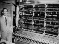
John von Neumann and the ENIAC computer.
John von Neumann, the developer of that first computer (called the ENIAC), recognized that the problem of weather forecasting was a natural for his computing machinery. In 1948, he assembled a group of theoretical meteorologists at the Institute of Advanced Study in Princeton, New Jersey. The group was headed by Jule Charney, who had done extensive work on developing a simplified, filtered system of equations for weather forecasting. His group constructed a successful mathematical model of the atmosphere and demonstrated the feasibility of numerical weather prediction.
The first one-day, nonlinear weather prediction was made in April, 1950. Its completion required the round-the-clock services of the modelers, and, because of several ENIAC breakdowns, more than 24 hours to execute. However, this first forecast was successful in proving to the meteorological community that numerical weather prediction was feasible.
Creation of the Joint Numerical Weather Prediction Unit
By 1954, both modeling capability and computer power had advanced to a point where the possibility of real-time operational numerical weather prediction was under active consideration in Europe and the United States. On July 1, 1954, the Joint Numerical Weather Prediction Unit (JNWPU) was organized, staffed, and funded by the U.S. Weather Bureau, the U.S. Air Force, and the U.S. Navy. This new unit was given the mission to apply emerging computer technology to the operational production of weather forecasts.
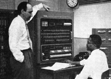
Fred Shuman (left) and Otha Fuller, circa 1955 at the IBM 701. The 701 was the first computer used by the JNWPU to produce operational numerical weather prediction. Click image for larger view.
Using a newly purchased IBM 701, by mid-1955, the JNWPU was issuing numerical weather predictions twice a day. These early forecasts offered no competition for the ones being produced manually. However, the operational environment in which the forecasts were produced provided the necessary impetus to rapidly identify modeling problems and implement practical solutions. By 1958, the forecasts being produced began to show steadily increasing and useful skill.
Continued Evolution of Numerical Weather Prediction
The evolution of numerical weather prediction throughout the latter part of the 20th century proceeded at a similar pace at many operational numerical weather prediction centers around the globe. The first numerical weather prediction models used in the United States ran on grids that covered the Northern Hemisphere. This restriction was based primarily on the amount of computer power as well as the amount of data available to initialize the model. However, a progression of more and more powerful computers procured by the National Weather Service throughout the 1960s and 1970s as well as increasing sources of data—particularly from weather satellites—allowed the expansion of both the domains and the number of models run.
Increases were also made in the number of vertical levels and the horizontal resolution of the models. A three-layer hemispheric model was introduced in 1962 and a six-layer primitive equation model appeared in 1966. Additional atmospheric layers allowed more accurate forecasts of winds and temperature, resulting in better prediction of storm motion.
The first regional system concentrating on North America, called the Limited Fine Mesh model, was implemented in 1971. The first global model became operational in 1974.
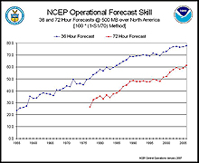
This graph shows computer power and time versus model accuracy as defined by the S1 score (a measure of the skill of the forecast) of 36- and 72-hour NCEP 500-millibar forecasts. Click image for larger view.
The late 1970s and the 1980s saw the introduction of the use of spectral coordinates and advances in methods of data assimilation and more accurate representation of physical processes in the atmosphere such as the formation of clouds and precipitation. During the 1990s, models of finer and finer scales were developed.
A more recent addition to the numerical weather prediction suite of products is “ensemble modeling.” With ensemble modeling, many forecasts are run with slightly varying initial conditions from different models and an average, or "ensemble mean," of the different forecasts is created. This ensemble mean can extend forecast skill to the two-week range because it averages over the many possible initial states, to essentially “smooth” the chaotic nature of the atmosphere. In addition, this technique provides information about the level of uncertainty for different conditions because of the large ensemble of forecasts available.
All of the development during the 1960s – 1990s meant computer resources were stretched to the limit. As soon as new computer resources became available, they were fully utilized with higher-resolution models with improved representation of physical processes, using more and more sophisticated and complex modeling techniques and an increasingly larger number of observations from around the globe, especially from satellites. Advances in predictive skill could be shown to be directly proportional to advances in computing and modeling.
However, the computer-based forecast is not the only reason for the improvements in forecasting accuracy the world enjoys today. The interpretation of the model forecasts by human forecasters has been shown to provide a consistent amount of additional forecast improvement throughout the evolution of numerical weather prediction. Our ability to interpret the many “moods” of the atmosphere has not yet been matched by equations and computer chips.
Numerical Weather Prediction Today
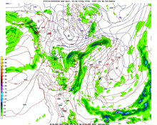
A 48-hour forecast from NCEP’s North American Mesoscale (NAM) model showing mean sea level pressure (solid lines) in millibars (mb), 1000-500 mb thickness (a measure of temperature of a layer) in decameters (red and blue dotted lines), and six-hour total precipitation in inches (colored contours using scale on left). The forecast was valid May 24, 2007. Click image for larger view.
In the present day, operational numerical weather prediction centers around the globe run a myriad of models. These models, some of which were developed and are run by NOAA’s National Weather Service, produce a wide variety of products and services. In the United States, over 210 million observations, the vast majority obtained from satellites, are processed and used each day as input into global and regional models producing forecasts for atmospheric and oceanic parameters, hurricanes, severe weather, aviation weather, fire weather, volcanic ash, air quality, and dispersion. The current operational computers run with a sustained computational speed of 14 trillion calculations per second. More than 14.8 million model fields are generated every day, six million of which are derived from the global ensemble runs.
In 2005, the first dynamic climate forecast system was implemented, making forecasts out to one year. Models that predict space weather on an operational basis are not far off. Demands for more and more detailed weather information increase on a regular basis.
Looking Ahead
The future holds more areas for progress in environmental modeling. An Earth systems modeling approach offers a way to couple models from oceanic, land, cryospheric (ice), and atmospheric disciplines in order to transfer information among model components. The suite of forecast products will expand beyond weather, water, and climate services to include ecosystems and incorporate the needs of more customers, such as the transportation, health, and energy communities.
Numerical weather prediction has advanced significantly since the idea was formed by Bjerknes and tested by Richardson. The six weeks of tedious computations endured by Richardson can now be done in the blink of an eye. The past century’s efforts have resulted in a level of accuracy for weather prediction that saves countless lives and property each year. Numerical weather prediction can indeed be considered one of the most significant achievements of the 20th century.
