
Making the Map
From the start of aerial photography in the Coast and Geodetic Survey (C&GS) Coastal Mapping Program in the 1920s, there have been many methods devised, and devices constructed, to make maps from aerial photographs. Overall, the mapping methods fall into three main groups: graphic, analog stereoscopic, and analytical stereoscopic.
The Graphic Way
Graphic map compilation methods are relatively simple. They rely on having a large number of ground control points (points with known locations on the Earth) visible in the photographs.
The control points are surveyed in the field to determine their coordinates (latitude and longitude), and then marked on a map sheet. The transparent map sheet is positioned on top of a photograph (or a mosaic of several photographs), and a group of the marked control points on the sheet are lined up with their corresponding points in the image. The map can only be lined up with one portion of the photo at a time, because of various distortions in the photographic image.
Next, the details in that area of the photo are traced from the photo onto the map sheet. The map is then shifted to align a different group of control points with their corresponding points in the image, and the details in that area are then traced. This procedure is followed until the entire map sheet has been compiled.
The graphic method works best in flat areas of land and where the camera was not tilted far from vertical when the photos were taken. When the area being mapped was hilly, then more control points were required, and only small areas of the photo could be traced before the map had to be adjusted.
Fortunately, many parts of the U.S., especially in the southeast and Gulf states, are quite flat. Graphic map compilation was used in the earliest C&GS aerial photo projects in New Jersey, Florida, and Louisiana. This method continued to be used for many years, especially with revisions of previous surveys (where plenty of existing control points were available) and in flat areas where the mapping of topographic contours (elevation lines) was not required.
Seeing In Stereo

This stereogram shows two overhead images, taken from two different perspectives, of a lake, stream valleys, and surrounding hills. If you center yourself in front of the images, relax your eyes, and try to stare through the image, as if looking into the distance, you might be able to combine the two images into a single 3-D view of the terrain. It could be easier to first try merging the two white circles above the images into one combined circle in the center, and then slowly letting your eyes slide down for a 3-D image of the terrain.
Many areas of the country are not flat, especially along the West coast and throughout Alaska. In the most mountainous areas, it was very difficult to survey many control points. A way was needed to compensate for the variations in height of the terrain, for the tilt of the camera, and the distortions of the lens and film. Fortunately, the principles of how to make compensations were well understood by the end of the 19th century, well before the Coast Survey started experimenting with aerial photography.
In Europe, various instruments for making accurate measurements and compiling maps from photographs were developed in parallel with advances in photographic technology. Practically all of these instruments were designed to work with strips of overlapping photographs, where part of the image in one photo also appears in the next photo of the strip. When the two photographs are arranged such that the left eye views one photo, and the right eye views the other, an object in the overlap area can appear to have height or depth. The combined image that you see with both eyes is called a “stereo-model.”
Along with the concept of stereo viewing, these photogrammetric instruments (as they came to be called) also used the principle of the “floating mark”. This was simply a measuring mark (usually a black dot) superimposed on the views of the left and right images. Using the controls of the instrument, the mark could be made to move about the stereo-model and its apparent elevation could be adjusted to follow the hills and valleys of the terrain in the scene. Various methods were used to remove the effects of camera tilt and differences in scale between the photographs. Attached to the stereoscopic instrument was a drawing or plotting device that was used to mark lines or points on a map sheet as the floating mark was moved about the stereo-model.
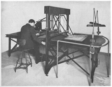
In 1939, the Model A Reading plotter was built. This stereoplotter, based on a design by Lieutenant Commander O. S. Reading, was the first instrument that was compatible with the C&GS nine-lens camera. Click image for larger view.
Many varieties of these photogrammetric instruments were designed and built in Europe, Canada, and the U.S. Some were more complex and costly than others. Generally, the more complicated and expensive the instrument was, the more accurate the final results. Many models could only be used with photos from a particular type of camera or lens.
The C&GS nine-lens camera was a device with unique characteristics used by C&GS in the 1940s, 50s, and 60s. Photographs from this camera were not compatible with any existing stereo plotting instruments. In 1939, a stereoplotter for the nine-lens photography was built.
By 1949, the C&GS Photogrammetry Division owned at least 18 different types of stereoscopic plotting instruments of varying complexity. All but the Reading plotters used only single-lens photography.
The analog stereoplotter instruments were used until the late 1980s, when they were replaced by analytical plotters.
Going Digital
The analytical stereoplotter is a high precision universal stereoscopic mapping and aerotriangulation system. Analog plotters used purely optical and mechanical devices to simulate the stereo-model and compensate for the distortions in the photographic imagery. In contrast, the analytical plotters use computers to mathematically solve for the parameters of the photogrammetric equations and determine the mechanical adjustments required for the instrument to form the stereo-model, while correcting for all known sources of error. This advancement was made possible by the development of the computer in the late 1950s and early 1960s.
The analytical plotter was a quantum leap in sophistication that allowed photogrammetric mapping to become more flexible and accurate than ever before. The analytical plotters, being universal machines, were much less limited by the mechanical constraints of the instruments. A broader range of photographic formats, scales, focal lengths, camera tilts, and distortions of many types could be handled by a single instrument.
In the late 1980s, the National Ocean Service (of which the C&GS was now a part) commissioned to have an analytical plotter built to C&GS specifications. It was aptly called the NOSAP. Soon after, additional analytical plotters were purchased, and eventually all coastal mapping was being conducted on the new instruments.
The modern era had begun.